Build the most powerful hypothesis test: Part 2

In the post Build the most power hypothesis test: Part 1 we introduced Neyman-Pearson criterion and Sufficient Statistic. In this post, using both of these ideas we will develop an optimum decision rule. To interactively generate likelihood functions and see the impact of choosing , do not forget to try the Shiny app linked in this post.

Finding the Optimum Decision Rule:

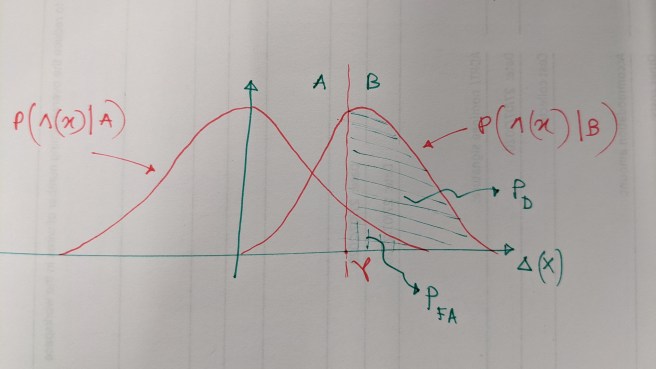
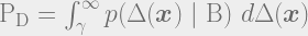
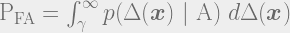
This is a futile attempt to draw the likelihood functions of under each hypothesis. The vertical line at is a decision rule (or threshold in this case) and it divides the region over which the likelihood functions are defined into two disjoint region. Notice an interesting thing. If you slide the threshold to the right, will be reduced, but probability of correct detection will reduce as well! If you slide it to the left, you will end up with higher probability of correct detection but at the cost of enhanced probability of false alarm. This is a fundamental trade-off in hypothesis testing and fortunately, this trade-off is at the discretion of those who designs the test. From the figure, it is clear that the given will yield a fixed position along the axis which means . It consequently results into the following :

It is obvious that we cannot obtain a higher than this. Hence is our optimum decision rule.

As a matter of fact, we have maximized probability of correct decision for a given probability of false alarm which is the problem outlined in (7) in Part 1. For convenience, the problem statement is restated below:

… (7)

I am skipping the description about the relationship between and . Do not worry, the mathematics behind that is not hard at all and it is fun to derive.

Now, for a given , the Neyman-Pearson criterion looks for the by solving the following

So far, we have dealt with an extremely simple example. We considerd that the likelihood functions under each hypothesis are Gaussian with different mean but share the same variance. One of the most common scenarios is having Gaussian random variables under each hypothesis which share the same mean but have different variances. In that case, the sufficient statistic is no longer Gaussian, rather it becomes scaled Chi-square random variable with degree of freedom under each hypothesis. Try it, that’s fun!

Evaluating the Test Performance:

Since, the choice of is pre-specified and directly influences , it is important to assess how this choice impacts the probability of correct decision. This is done with the help of a parametric plot known as Receiver Operation Characteristic (ROC), which is a parametric plot.

Click here to interact with the Shiny-app that generates ROC for two given Gaussian likelihood functions under null-hypothesis and alternative hypothesis. The Gaussian likelihood function under null-hypothesis is kept fixed at zero mean while the mean of the likelihood under alternative hypothesis can be changed using the Mean of Gaussian Observation slider. You can also change using the slider Probability of False Alarm. You will notice that, the ROC moves toward the (1,0) corner of the plot as the separation between two hypothesized model increased. On the other hand, it tries to land on line as the overlap between these two function increases.

The choice of is case specific. An example is: probability of miss detection plays crucial role in a missile detection system. A miss detection can lead to catastrophes at large scale. On the other hand, a false alarm can be dealt via further investigation on the signal. In this case, the test designer should prioritiize while putting less concern on .

I hope this two-part series served you well to grow an instinct about how hypothesis testing works, how we can develop optimum decision rule and how we can decide about pre-specified . Thank you!

(The comic in the featured image is stolen from the amazing xkcd)