
(This blog has already been appeared at my Medium and can be found here. Later, Analytics Vidhya published it under their publication as well.)
Fourier Transform is undoubtedly one of the most valuable weapons you can have in your arsenal to attack a wide range of problems. FFT is literally the bread and butter for many signal processing engineers. At the same time, there are examples of application of FFT in data science realm. For example, time-series data with dense interval (for example: instead of monthly sales data, you might be dealing with hourly sales data) exhibits complex seasonality. Fourier Transform is a handy tool to analyze the seasonalities of those kinds. Unfortunately, in an inexperienced hand, it can lead to disastrous and frustrating conclusions sometimes.
I was surfing through hundreds of discussions and Q&A in stack-exchange, Mathworks and other forums. What I have learned is: people who intend to use Fourier Transform do know why they want to use it. But the common confusion is: What’s next? How to “post-process” the sequence in hand and get a meaningful and accurate insight? To be more specific, there are mainly following questions:
- What is Single Side Band (SSB)? Why do we care?
- What is the relationship between my FFT sequences and physical frequencies? How these two can be correctly aligned?
- What is FFT bins? How does it set the resolution of FFT?
- Why there is a normalization factor?
The source of confusions are buried beneath the mathematical fundamentals which built the foundation of Fourier Transform. In this article, I will try to breakdown several common confusions which arise while working with Fourier Transform. I will try to explain the reasoning using as little mathematics as possible. Hopefully this will help you to work with this amazing tool without going through the trouble of picking up the mathematics behind it.
For explanation, I will be using an example code for Fast Fourier Transform (FFT). FFT is essentially a super fast algorithm that computes Discrete Fourier Transform (DFT). The example code is written in MATLAB (or OCTAVE) and it is a quite well known example to the people who are trying to understand Fourier Transform. Similar example can be found in here.
In what follows next, we will be taking parts from this code and analyze it. First, let us set up the context. We have a sampler which can sample 1000 samples in a second. We have gathered 500 time points using that sampler.
Fs = 1000; %sampling rate
T = 1/Fs; %sampling interval
L = 500; %Number of time points
t = 0:T:(L-1)*T; %time vector
Next, let us create a signal with 3 frequencies and a DC component (component with 0 Hz) which will be sampled. Let us add some noise as well. If you want, you can plot your signal for an initial visual inspection. That’s a good practice.
% Define frequencies
f1 = 20;
f2 = 220;
f3 = 138;
% Create the signal
x = 5 + 12*sin(2*pi*f1*t-0.3) + 5*sin(2*pi*f2*t-0.5) + 4*sin(2*pi*f3*t - 1.5);
x = awgn(x,5,'measured') %noise with 5 dB Signal to Noise ratio
Now, we are all set for performing FFT. We have a real world signal in our hand which is a mixture of sinusoids corrupted by additive noise. Let us take the FFT and plot it. Bummer. Oh yes, FFT sequences are complex sequences. Why? Because they contain information about amplitude and phase for a given frequency component and complex numbers are the best way to describe it. Let us take the absolute value (magnitude) of those sequences then. What do we get?
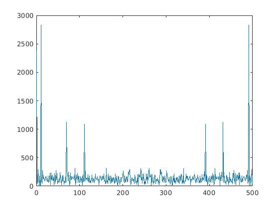
This do not make much sense at all. First of all, there are 7 peaks (including the one at zero). But we were expecting 4 peaks, (3 for frequencies f1,f2,f3 and 1 for the DC component). Secondly, what has happened to the amplitude? It looks too high! The peaks are in wrong place as well. It is pretty evident that to work with this thing, we have works to do.
Let us break the first confusion: why there are more peaks than we were expecting? This is where Single Side Band (SSB) spectrum comes to play. If you look closely, one side of the plot above is the mirror reflection of another side, dropping the peak at 0. This is because, for real signals, the coefficients of positive and negative frequencies become complex conjugates. That means, we do not need both sides of spectrum to represent the signal, a single side will do. This is known as Single Side Band (SSB) spectrum. To get the SSB spectrum, we need transform our time domain signal into the analytic signal which is xₐ = x + iH(x). H(x) is the well known Hilbert Transform. But, the good news is- we do not need to learn a new transform for that. It turns out, if you take the spectrum associated with positive frequencies only and multiply it by 2, you will get the SSB spectrum without explicitly applying Hilbert Transform on converted analytic signal. This can be done simply writing the two lines of additional code as shown in the following snippet:
X = fft(x,N);
SSB = X(1:L/2);
SSB(2:end) = 2*SSB(2:end);
Note that, we excluded the first element while multiplying by 2. This is because, in MATLAB, the FFT function returns a vector where the first element is the DC component (associated with 0 frequency). A DC component is associated with 0 frequency, which is neither positive nor negative. In reality, this coefficient is real.
Next, we need to fix an appropriate x-axis for the FFT spectrum. In our case, we need to put the physical frequencies in the x-axis so that we know we are getting peaks at the correct frequencies. This is an extremely crucial step. To do that, we need to understand how FFT creates “bins”. For N point FFT, the number of bins created is N/2.
FFT is just an implementation of Discrete Fourier Transform (DFT). To discretize the continuum of frequencies, the frequency axis is evenly segmented into finite number of parts which are known an bins. Bins can be considered as spectrum samples. In our example, the sampling frequency Fs = 1000 samples/second. According to Nyquist law, the highest physical frequency which can be represented by its samples without aliasing is simply Fs/2 = 500 Hz. So, essentially the frequency spectrum is being segmented into strips of (Fs/2)/(N/2) or Fs/N bins. This is big. We can now create appropriate frequency axis as shown in the snippet below.
f = (0:N/2-1)*(Fs/N);
Moreover, bins give us the idea about the underlying frequency resolution of FFT. In a simpler word- to which extent we will be able to separate two closely placed frequencies in the spectrum. In our example, our frequency resolution is Fs/N = 1000/1024 or 0.9765 Hz/bin. We won’t be able to separate frequencies as distinct peaks if they have a spearation less than 0.9765 Hz.
We are almost there. We have extracted the Single Side Band spectrum. We also have established the axis of the spectrum. Now, we want to simply look at the spectrum and spell out the amplitudes of each sinusoids. Before doing that, let me rephrase DFT a little bit. Remeber the definition of DFT?

If you look closely, you will notice that, computing DFT ressembles correlation a lot. That’s right. In fact, I think this is a great intuitive way of thinking about how DFT works. So, essentially for each bin, we compute the cross-correlation between our time domain signal x and a complex sinusoid associated with that bin. A further investigation reveals that, something is indeed missing which we usually see along with a correlation operation. A normalization factor. To be specific, a normalization factor of signal length. That’s what we will do, we will normalize the spectrum with signal length. Now, let us put all of these understandings together and let us see what happens.
figure(4)
plot(f,abs(SSB/L)) %Normalizing with signal length
xlabel('f (in Hz)')
ylabel('|X(f)|')
title('Corrected Frequency Spectrum')

Voila! We have successfully retrieved our frequencies from deep beneath the noise. I suggest you to play with the code attached and see what happens at different signal length, FFT points and frequencies. I would like to remind you that, for given settings in the code, aliasing will happen if you chose a frequency above Fs/2. Frequencies higher than Fs/2 will appear as a low frequency component in the spectrum because of aliasing. That is why, a low-pass filtering is suggested before applying FFT, especially if you do not have any knowledge about the potential frequency components of your signal.
I hope this story will equip you with some basic understanding about handling FFT operations. For the ease of explanation, many of mathematical perspectives are oversimplified since I am trying to cater a broad class of readers. See you next time!
(The featured image was taken from xkcd. This site is an absolute gem of nerdy humor, do check it out.)
