Randomized SVD with Power Iterations for Large Data Matrices

What is Randomized SVD?

Few days ago, I happened to come across a question in a forum. Someone was asking for help about how to perform singular value decomposition (SVD) on an extremely large matrix. To sum up, the question was roughly something like following

“I have a matrix of size 271520*225. I want to extract the singular matrices and singular values from it but my compiler says it would take half terabyte of RAM…”

Half terabyte of RAM. No jokes here. However, this particular question is becoming relevant day by day because of the abundance of data we are experiencing now a days. For example, improved sensors in our smartphone cameras or streaming HD videos in YouTube. We are increasingly facing scenarios where we need to deal with millions of measurements and even larger number data points in real time, given limited computational resource or strict latency requirement. On top of this, another two questions remain. The first one is: does the intrinsic rank or information captured by these measurements also scales up at the same rate with the number of measurements? The answer is, often, NO. Then the next question is: if the intrinsic rank is small, can we do SVD in a computationally efficient manner?

SVD is known as the Swiss army knife of linear algebra. I personally think it is a wrong way of advertising it. It often makes people agnostic about the overhead it requires and leads to situations like above. In this blog, we will be examining the bottlenecks of applying SVD on extremely large datasets. Then we will see, how the elegant theorems from random matrix theory can provide us tools to deal with those bottlenecks efficiently and lead us to highly accurate yet computationally efficient approximation of our data matrix.

Let us consider a tall, rectangular data matrix $\mathbf{S} \in \mathbb{R}^{p\times q}$ where $p>>q$ . We have $q$ data points for $p$ features. SVD decomposes this humongous matrix into three matrices, two of them contain left and right singular vectors respectively and one of them contains the singular values, diagonally arranged in descending order.

$\mathbf{S} = \mathbf{U}\mathbf{E}\mathbf{V}^*$ … (1)

where, $\mathbf{U}\in\mathbb{R}^{p\times p}$ and $\mathbf{V}\in\mathbb{R}^{q\times q}$ . $\mathbf{E}\in\mathbb{R}^{p\times q}$ is a non-square diagonal matrix. Almost surely $\mathbf{S}$ is a full column rank matrix, hence it has only $q$ non-zero singular values.

In this specific case, the bottleneck I was talking about is essentially the computation of the matrix of left singular vector $\mathbf{U}$ because of its dimension $p\times p$ . As a matter of fact, now we can update our objective as following

How we can come up with a low cost yet accurate approximation of $\mathbf{U}$ ?

We turn into random matrix theory to find the answer this question. It tells us that- if we randomly sample the column space of our original data matrix $\mathbf{S}$ by taking random projections, it is highly unlikely that the projection will throw away any important part of the story being told by the data matrix. The idea of random projection is largely based on the famous Johnson-Lindenstrauss Lemma. If we fix a target rank $r<q$ , then we can take a random projection of our data matrix:

$\mathbf{T} = \mathbf{S}\mathbf{\Omega}$ … (2)

where $\mathbf{\Omega} \in \mathbb{R}^{q\times r}$ is the random projection matrix. It can be a Gaussian random matrix for example. The selection of random matrix is a different study in its own right, hence I am omitting the details here for brevity. Now, the projected matrix $\mathbf{T} \in \mathbb{R}^{p\times r}$ approximates the columns space of original data matrix $\mathbf{S}$ almost surely. So, if we want to find a set of orthonormal bases of $\mathbf{S}$ , it is enough to perform QR decomposition on $\mathbf{T}$ instead of $\mathbf{S}$ !

$\mathbf{T} = \mathbf{Q}\mathbf{R}$ … (3)

Note that, now we have the orthonormal bases for the $r$ -rank approximation of $\mathbf{S}$ . Now we take another projection of $\mathbf{S}$ , but this time on the subspace spanned by the orthonormal matrix $\mathbf{Q}$ .

$\mathbf{\Upsilon} = \mathbf{Q}^*\mathbf{S}$ … (4)

where $\mathbf{\Upsilon}$ has a dimension of $r\times q$ .

One of the serious advantage offered by SVD is, it is generalized for data matrix of any dimension, unlike Eigen-decomposition which works only on square matrices. That is not the end of the story. The left singular vectors are essentially the eigenvectors of $\mathbf{S}\mathbf{S}^*$ . On the other hand, the right singular vectors are the eigenvectors of $\mathbf{S}^*\mathbf{S}$ . Note that,

$\mathbf{\Upsilon}^*\mathbf{\Upsilon} = \mathbf{S}^*\mathbf{Q}\mathbf{Q}^*\mathbf{S} = \mathbf{S}^*\mathbf{S}$ … (5)

Since $\mathbf{Q}$ is orthonormal, $\mathbf{Q}^*\mathbf{Q} = \mathbf{Q}\mathbf{Q}^* = \mathbf{I}$ . Since, $\mathbf{S}\mathbf{S}^*$ and $\mathbf{S}^*\mathbf{S}$ share the same set of eigenvalues while the singular values are simply squared eigenvalues of these matrices. This means, if we take the SVD of $\mathbf{\Upsilon}$ , then the corresponding singular values and right singular vectors will be same as provided by $\mathbf{E}$ and $\mathbf{V}^*$ in Equation (1) respectively!

$\mathbf{\Upsilon} = \overline{\mathbf{U}}\mathbf{E}\mathbf{V}^*$ … (6)

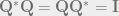
Now, we can compute the high dimensional left singular matrix using the simple matrix-vector multiplication

$\mathbf{U} = \mathbf{Q}\overline{\mathbf{U}}$ … (7)

The Role of Power Iterations

Power Iterations is a very well known framework for those who are familiar with how recommendation system works. Like randomized SVD, power iteration also has its root in random matrix theory. Upon its initialization with a unit norm random vector, It iteratively computes the dominant eigenvalue of a square matrix. It plays crucial role in Google’s PageRank algorithm. Moreover, Twitter’s WTF (Who to Follow) algorithm is essentially based on power iterations.

In our venture here, however, we are not interested in computing the dominant eigenvalue. Remember our target rank $r$ in previous section? I did not specify any strategy about choosing a target rank there because it depends on circumstances. What if our chosen target rank $r$ is smaller than the intrinsic rank and we end up throwing significant amount of variance away? Another way of describing this phenomenon is – what if the singular values of our data matrix $\mathbf{S}$ decay very slowly?

In that case, we can preprocess our data matrix $\mathbf{S}$ using power iteration. Let us define $\mathbf{\Delta} = \mathbf{S}\mathbf{S}^*$ . From the property of eigen decomposition, we know that

$\mathbf{\Delta}^{(i)} = \mathbf{X}\mathbf{\Phi}^{(i)}\mathbf{X}^{*}$ … (8)

The superscript $(i)$ here means the $i^{th}$ power. Now, if we do the following

$\mathbf{S}^{(i)} = \mathbf{\Delta}^{(i)}\mathbf{S}$ … (9)

it can be easily shown that we will get the following

$\mathbf{S}^{(i)} = \mathbf{U}\mathbf{E}^{2r-1}\mathbf{V}^*$ … (10)

The processed data matrix $\mathbf{S}^{(i)}$ now has much faster decaying singular value spectrum. It can give us a dramatic improvement in approximating conventional SVD, however, at the cost of additional computation. In practice, it is absolutely suicidal (and pointless) to do power iteration by raising the power of $\mathbf{\Delta}$ . One of the staple methods of raising power of a matrix is to perform eigen decompostion first, then simply raise the powers of its eigenvalues. But the eigenvectors of $\mathbf{\Delta}$ are the left singular vector of our data matrix, which we are looking for. An intelligent way of avoiding this perpetual calculation is to take the random projection first, then multiply it with $\mathbf{S}^*$ and $\mathbf{S}$ alternatively.

One of the most beautiful thing about randomized SVD is the existence of closed-form lower bound of approximation error as a function of target rank $r$ and the degree of power iteration $i$ . Hence, you can trade-off between approximation performance and computational requirement easily. More on this topic can be found in this amazing paper.

Example

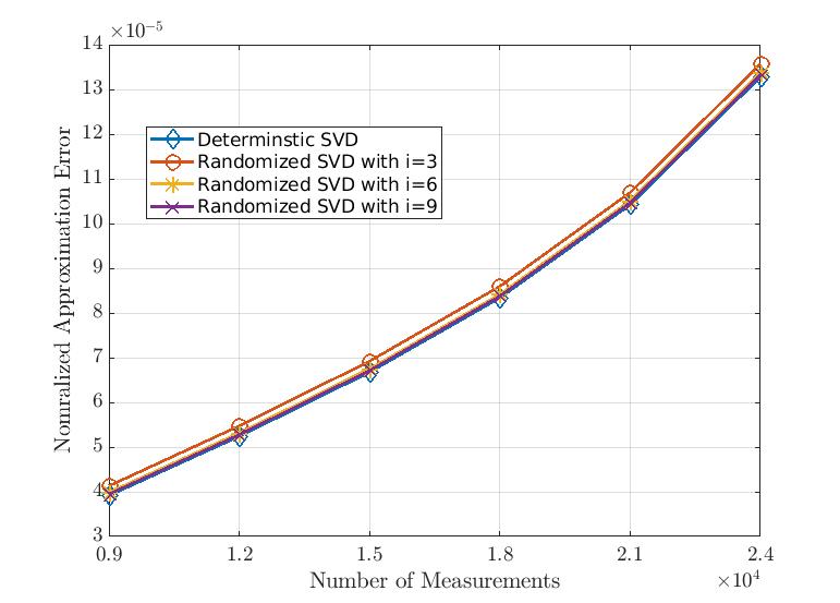
In this plot, we can see how good randomized SVD can approximate our data matrix with increasing number of measurements (or features) for a given number of data points. Here, we fix the number of data points as 3000 and vary the number of measurements from 9000 to 24000. We also set the target rank as 10% of number of measurements. Moreover, in this example, $i$ is the number of power iteration. It is evident, the randomized SVD can almost attain the low-rank approximation performance of conventional deterministic SVD.

Next, we have the algorithm runtime shown in the plot above. Using only 3 power iterations, we can have really good approximation of data matrix using only half of the computational resources required by deterministic SVD!

I have created a gist in github to share the reproducible codes used in this example.

	clc;
	close all;
	clear all;

	%% Creating a large dataset
	measurement = 9000:3000:24000;
	lp = length(measurement);
	dtime = zeros(lp,1);
	derror = zeros(lp,1);
	rtime = zeros(lp,3);
	rerror = zeros(lp,3);
	for i=1:length(measurement)
	SS = randn(measurement(i),3000);
	tstart = tic;
	[U,E,V] = svd(SS);
	r = 0.1*size(SS,1); % target rank
	det_SVD = U(:,1:r)E(1:r,1:r)V(:,1:r)';
	dtime(i) = toc(tstart);
	derror(i) = 1/(size(SS,1)size(SS,2))norm(det_SVD – SS,'fro');
	%% Preprocessing
	% Select degree of power iteration
	index = 1;
	for q=3:3:9
	tstart = tic;
	% Create a random projection
	omega = normrnd(0,1/sqrt(size(SS,2)),size(SS,2),r);
	% Taking the random projection
	T = SS*omega;
	% Power iteration
	for iter = 1:q
	T = SS(SS'T);
	end

	%% Random SVD

	% QR Decomposition
	[Q,R] = qr(T,0); % economy QR decomposition
	% Project SS to Q
	gamma = Q'*SS;
	% randomized SVD
	[UU,E,V] = svd(gamma,'econ');
	U = Q*UU;
	rtime(i,index) = toc(tstart);

	%Reconstruct reduced rank data
	rand_SVD = Q*gamma;
	rerror(i,index) = 1/(size(SS,1)size(SS,2))norm(SS – rand_SVD,'fro');
	index = index + 1;
	end
	end
	set(groot, 'defaultAxesTickLabelInterpreter','latex'); set(groot, 'defaultLegendInterpreter','tex');
	figure(1)
	plot(measurement, sort(dtime))
	xlabel('Number of Measurements','interpreter','latex')
	ylabel('Runtime (in seconds)','interpreter','latex')
	hold on
	plot(measurement, sort(rtime(:,1)))
	hold on
	plot(measurement, sort(rtime(:,2)))
	hold on
	plot(measurement, sort(rtime(:,3)))
	figure(2)
	plot(measurement, sort(derror))
	xlabel('Number of Measurements','interpreter','latex')
	ylabel('Nomralized Approximation Error','interpreter','latex')
	hold on
	plot(measurement, sort(rerror(:,1)))
	hold on
	plot(measurement, sort(rerror(:,2)))
	hold on
	plot(measurement, sort(rerror(:,3)))

view raw random_svd_example.m hosted with ❤ by GitHub

I hope this blog will help you to get a surface level understanding about how randomization plays role in dealing with extremely large datasets.

(The feature image credit goes to the amazing xkcd comics).

Randomized SVD with Power Iterations for Large Data Matrices

Published by Shah Mahdi Hasan

Leave a Reply Cancel reply

Share this:

Like this:

Related

Published by Shah Mahdi Hasan

Leave a Reply Cancel reply